Why Metropolis works
Building intuition for MCMC
Markov Chain Monte Carlo (MCMC) is a common tool for sampling from complex distributions. In the machine learning and data science world, MCMC is sometimes used to get distributions over parameter variables for Bayesian models. Because MCMC methods can be easy to implement, it’s possible to apply these sampling procedures without understanding the bigger picture. This tutorial focuses on developing intuition for the basic idea underlying MCMC. Other resources include more techincal detail if you get hooked.
In general, MCMC algorithms allow you to sample from any target distribution . We typically don't know how to just draw samples tractably from . Otherwise we'd just sample from and observe its distribution, which is what we are trying to figure out in the first place! However, we can usually compute up to some normalizing constant , meaning that if , we can usually compute the numerator really quickly, even if computing is hard or slow.
I'll focus on one simple MCMC method, the Metropolis algorithm. Each iteration of Metropolis consists of two steps. In the first step, you make a proposal to move from state to state . You’re allowed to pick any proposal distribution that you want, so long as the probability of moving from to is equal to the probabilty of moving from to , which can be written , and so long as has some chance of moving to all non-zero regions of . In the second step, you accept the proposal with a probability defined by this seemingly odd rule:
where I use \(A(x' \vert x)\) to denote the probability of accepting the move from \(x\) to \(x'\). If you look closely at this (somewhat unintuitive) equation, you will see that if \(p^*(x)\) is bigger than \(p(x')\), you accept the proposal to move from \(x\) to \(x'\) with probability \(\frac{p^*(x’)}{p^*(x)}\). But if \(x'\) is bigger, the fraction will be bigger than 1, and you just move to \(x'\) automatically (i.e. with probability 1).
When I first learned about Metropolis I found it quite surprising, especially since you can pick (basically) any proposal \(Q\) that you want. This procedure allows you to draw samples from any ? Why does it work?
Sampling from a Markov chain
Let’s ignore Metropolis for a minute and imagine that we have a Markov chain with two states \(a\) and \(b\), where \(a\) transitions to \(b\) with probability 1 and \(b\) transitions to \(a\) with probability .5, and \(b\) remains in \(b\) with probability .5. I’ll use \(T\) to denote the probability of transitioning from one state to another. For instance, in this case \(T(a \vert b)\) = .5, \(T(b \vert b)\) = .5 and \(T(b \vert a) = 1\).
We can imagine that that if we “run” this Markov chain for many steps (i.e. keep sampling the next state), it will eventualy reach a stationary equillibrium, where on average it spends some of its time in state \(a\) and some of its time in state \(b\).
I will use \(\pi\) to denote the probability of being in some state in the stationary distribution, e.g. \(\pi(a)\) is the probability of being in state \(a\). One way to estimate \(\pi\) is just to “run” the Markov chain for a number of steps (i.e. step through the chain, by sampling the next state) and observe often it spends in each state. For example, if we run this Python code to sample based on \(T\), we will find that \(\hat{\pi}(a) = .33\) and \(\hat{\pi}(b) = .66\), where \(\hat{\pi}\) represents our estimate of \(\pi\).
This simple idea underlies Markov Chain Monte Carlo methods, including the Metropolis algorithm. In MCMC, you define a Markov chain with a distribution over states \(\pi\) that is equal to \(p^*\). Then you just draw samples from the chain to estimate \(p^*\).
How do we find the right \(T\)?
The previous section explained how we can sample from some transition \(T\), in order to estimate some \(\pi\). This only works if we can find a \(T\) such that its stationary distribution \(\pi\) will be equal to \(p^*\), our target distribution. Expressed more mathematically, we need a \(T\) such that
which asserts that once \(T\) is in its stationary distribution \(\pi\), the probability of being in state \(y\) (i.e. \(\pi(y)\)) is the same as \(p^*(y)\), which is also the same as the probability of transitioning into state \(y\) at any given timestep under the stationary distribution.
It can be shown that if we have a \(T\) such that
for all states \(a\) and \(b\) then \(T\) fulfills the conditions in (1). It’s worth taking a second to build some intuitions for equation (2), which says that, for all \(a\) and \(b\), the probability mass flowing out from state \(a\) to state \(b\) is the same as the probability mass flowing from \(b\) to \(a\). When this occurs, \(p^*\) is said to satisfy “detailed balance” with respect to \(T\). (See this very nice, intuitive description of detailed balance).
You can prove that if some distribution satisfies detailed balance with respect to some \(T\), then it is the stationary distribution of \(T\). To me this seems very intuitive. If the probability mass going in to any given state is equal to the probability mass going out of any given state, the distribution will never change. The punchline is: if \(p^*\) satisfies detailed balance w.r.t. \(T\) then \(p^*\) is the stationary distribution of \(T\) and we can sample from \(T\) to sample from \(p*\).
Back to Metropolis
Recall the somewhat mysterious Metropolis update rule, which proposes a change from \(x\) to \(x'\), denoted \(Q(x' \vert x)\), and accepts the proposal with probability
\[A(x' \vert x) = min(1, \frac{p^*(x’)}{p^*(x)})\]which we are told will produce a sample from \(p^*\).
This equation makes a lot more sense if you recall that we are searching for a \(T\) such that
\[p^*(a)T(b \vert a) = p^*(b)T(a \vert b)\]for all states \(a\) and \(b\). Because \(p^*\) is what we are trying to sample from (and thus can’t change), we need to define some \(T(b \vert a)\) and \(T(a \vert b)\) so that the equation is true for all \(a\) and \(b\). Let’s rewrite the previous equation using the names \(x\) and \(x'\)
\[p^*(x')T(x \vert x') = p^*(x)T(x' \vert x)\]and denote each \(T\) as the product of two probabilities
\[p^*(x')A(x \vert x')Q(x \vert x') = p^*(x)A(x' \vert x)Q(x' \vert x)\]where we use \(Q(x \vert x')\) to refer to the probability of a proposed distribution from \(x\) to \(x'\) and use \(A(x \vert x')\) to refer to the probability of accepting the proposed move. Notice that now \(T(x \vert x')\)=\(Q(x \vert x')A(x \vert x')\), meaning you transition from \(x'\) to \(x\) if two things happen: you propose a move from \(x'\) to \(x\) and the move is accepted, each with some probability. If we rearrange a bit we have:
\[\frac{p^*(x')Q(x \vert x')}{p^*(x)Q(x' \vert x)} = \frac{A(x' \vert x)}{A(x \vert x')}\]Because \(Q(x \vert x') = Q(x' \vert x)\) (remember, the proposal is symmetric) we can simplify to
\[\frac{p^*(x')}{p^*(x)} = \frac{A(x' \vert x)}{A(x \vert x')}\]This is an equation with two unknowns, so there is no single solution. However, we are free to pick any \(A\) we want — so long as a given transition \(T(\cdot \vert \cdot)=Q(\cdot \vert \cdot)A(\cdot \vert \cdot)\) remains a valid probability, between 0 and 1.
Let’s consider two cases.
First, assume that \(p^*(x) > p^*(x')\) and therefore \(\frac{p^*(x')}{p^*(x)}\) is a valid probability. In this case, if we set \(A(x \vert x') = 1\) we get \(\frac{A(x' \vert x)}{1} = A(x' \vert x) = \frac{p^*(x')}{p^*(x)}\), which will be a number between 0 and 1. Thus \(T(x' \vert x) = Q(x'\vert x) \frac{p^*(x')}{p^*(x)}\) will be a valid probabilitiy for any pair, \(x\) and \(x'\).
Now let’s assume that \(p^*(x) < p^*(x')\). If so \(\frac{p^*(x')}{p^*(x)}\) will not be a valid probability, and if we set \(A(x' \vert x) = 1\) we will have
\[\frac{p^*(x')}{p^*(x)} = \frac{1}{A(x \vert x')}\] \[A(x \vert x') = \frac{p^*(x)}{p^*(x')}\]In either case, we have \(A(b \vert a) = \frac{p^*(b)}{p^*(a)}\) if \(p^*(a) > p^*(b)\) and \(A(b \vert a)=1\) if \(p^*(a) < p^*(b)\).
Another way to express all this, is that if we use a symmetric proposal distribution \(Q\) and transition from \(x\) to \(x'\) with probability
we will eventually reach a stationary distribution \(\pi=p^*\).
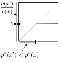
I find it helpful to imagine \(A\) as a threshold function, like the one below. If \(p^*(x') > p^*(x)\) then their ratio is a probability (the part of the graph that is climing) and we sample a transition from \(x\) to \(x'\) in proportion to their ratio. Otherwise, we transition from \(x\) to \(x'\) with probability one, meaning we always transition into the more probable state.
Another interpretation of \(A\) is that Metropolis always accepts moves into a more probable state, and sometimes accepts moves into a less probable state. In any event, I hope Metropolis is a bit less mysterious now.
One more important note
I’ve been writing \(p^*(x')\) this whole time. But remember (from way at the top of the post): we don’t know what \(p^*\) is, beyond that \(p^*(x)=\frac{\tilde{p}(x)}{Z}\). So we can’t actually compute (3) as written. However, because:
where \(\tilde{p}(x)\) is easy to compute and \(Z\) is hard, even if we don’t know \(\tilde{p}(x)\) we can still efficiently compute the ratio of \(p^*(x)\) and \(p^*(x)\), which is required for MCMC.
Thanks
Thanks to Javier Burroni for helping me better understand some of the mathematical details behind MCMC and providing a detailed technical edit. Thanks to Nick Eubank and Andrew Drozdov for their help presenting the material in this post.
Enjoy Reading This Article?
Here are some more articles you might like to read next: